Continuous Probability

For continuous sample spaces (like a dart hitting a target), we can’t list or count outcomes. Instead, probability is defined by area (or length, or volume).

Area-Based Probability

For a sample space Ω with total area A(Ω), the probability of any subset equals its share of the total area:

$$P(A) = \frac{\text{area of } A}{\text{area of } \Omega}$$

Equal areas mean equal probabilities. If one region has twice the area of another, it has twice the probability. This is the continuous analogue of “equally likely outcomes” — instead of each outcome being equally likely, each unit of area carries equal probability weight.

Example: Dart on a Unit Square

Throw a dart at a 1×1 square target. The sample space is Ω = {(x, y) : 0 ≤ x ≤ 1 and 0 ≤ y ≤ 1} — every point in the square is a possible outcome.

Question 1: What’s the probability of hitting the left half?

The left half has area 0.5, the whole square has area 1:

$$P(\text{left half}) = \frac{0.5}{1} = \frac{1}{2}$$

Question 2: What’s the probability of hitting a circle of radius 0.25 centered at (0.5, 0.5)?

$$P(\text{circle}) = \frac{\pi \cdot 0.25^2}{1} = \frac{\pi}{16} \approx 0.196$$

The Continuous Uniform Law

When every region of equal area has equal probability — no region is favored over any other — the model is called the Continuous Uniform Law. This is the continuous counterpart to the Discrete Uniform Law.

Example: A spinner points uniformly to a random angle from 0° to 360°. No part of the circle is favored over any other — so this is the continuous uniform law. Split the circle into 4 equal pie slices (0°–90°, 90°–180°, 180°–270°, 270°–360°). Each slice has the same area, so each has the same probability: $\frac{1}{4}$. This is exactly like splitting a fair deck of 52 cards into 4 suits — equal shares get equal probability. Count the cards for discrete, measure the area for continuous.

Not every continuous model is uniform — just like not every discrete model has equally likely outcomes. A dart thrown at a square with a bullseye in the center would favor the center region, so the uniform law wouldn’t apply. But when you have no reason to favor any region over another, the uniform law is the natural choice.

Individual Points Have Probability 0

What’s the probability of hitting exactly the point (0.3, 0.7)?

A single point has area 0, so:

$$P(\text{single point}) = \frac{0}{1} = 0$$

This is a key difference from discrete probability:

But a set of points can have positive probability — a region with area 0.3 has P = 0.3. Probability 0 for a single point doesn’t mean “impossible” in the everyday sense; it means the point takes up no area.

P = 0 Does Not Mean Impossible

After you throw the dart, it lands on some specific point. That point also had probability 0 before you threw — yet it happened. So in a continuous model, P = 0 does not mean impossible. It means you could never have predicted that exact outcome in advance, because a single point takes up no area.

The real tool for continuous probability is asking about regions, not exact points. “Will the dart land within 0.1 of (0.5, 0.5)?” has a positive probability. “Will it land exactly on (0.5, 0.5)?” has probability 0.

P = 1 Does Not Mean Certain

If P = 0 can still happen, then the complement can still fail. Consider the event “the dart lands anywhere except (0, 0)”:

$$\begin{aligned} P(\text{anywhere except } (0,0)) &= \frac{\text{area of whole square} - \text{area of one point}}{\text{area of whole square}} \\ &= \frac{1 - 0}{1} = 1 \end{aligned}$$

The probability is 1 — but it’s not guaranteed. The dart might still land on (0, 0). Removing a single point doesn’t change the area, so it doesn’t change the probability. But that point is still physically possible.

This only happens in continuous models. In a discrete model (like rolling a dice), P = 1 means every possible outcome is included — it’s truly certain. In a continuous model, P = 1 means “the area is fully covered,” but individual points contribute zero area, so removing one doesn’t change the total.

Example: Triangle in the Square

Back to the dart on the unit square. What’s the probability that x + y ≤ ½?

What does x + y ≤ ½ mean geometrically?

The equation x + y = ½ is a line. When x = 0, y = ½. When y = 0, x = ½. So this line connects the points (0, ½) and (½, 0) — it cuts across the bottom-left corner of the square.

The inequality x + y ≤ ½ means “all points on or below this line” — which forms a right triangle with vertices at (0, 0), (0, ½), and (½, 0).

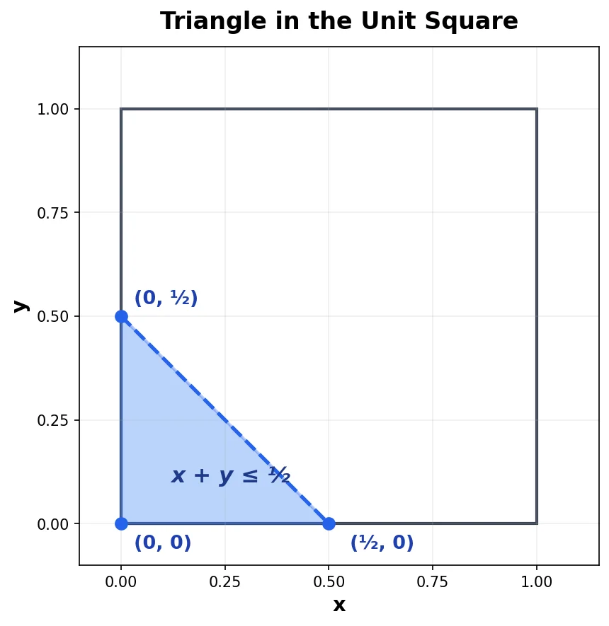
Step 1: Visualize the event. The condition x + y ≤ ½ defines this triangular region in the bottom-left corner of the square.

Step 2: Compute the area. The triangle has base ½ and height ½:

$$\text{Area} = \frac{1}{2} \times \frac{1}{2} \times \frac{1}{2} = \frac{1}{8}$$

Step 3: Divide by total area.

$$P(x + y \leq \tfrac{1}{2}) = \frac{1/8}{1} = \frac{1}{8}$$

This follows the same procedure as the discrete case — set up the sample space, identify the event, compute the probability. The only difference: area replaces counting.

Countable Additivity

The additivity axiom says: if A and B are disjoint events (no outcomes in common), then P(A ∪ B) = P(A) + P(B).

Example: Flip a coin until you get heads. Define:

• A = “first heads on flip 2”
• B = “first heads on flip 4”

These are disjoint — you can’t get your first heads on both flip 2 AND flip 4. Only one of them can happen. So P(A or B) = P(A) + P(B).

This works for any finite number of disjoint events. But what if we want the probability of “first heads on any even flip” — that’s flip 2, 4, 6, 8, and so on forever? That’s infinitely many disjoint events, and we can’t add them up with the finite axiom.

Countable additivity extends the axiom to this case: if you have infinitely many disjoint events that can be listed in order (first, second, third, …), then:

$$P(A_1 \text{ or } A_2 \text{ or } A_3 \text{ or } \cdots) = P(A_1) + P(A_2) + P(A_3) + \cdots$$

The subscripts just mean “the first event, the second event, the third event, …” — each one is a completely separate event, and they’re all disjoint from each other.

Why “countable”? Because the events must be listable — you can point to the first one, the second one, the third one. This covers finite lists (3 events) and infinite lists that go on forever (1, 2, 3, …). But it does not cover uncountable collections where you can’t even make a list.

Why the Limit Matters: The 1 = 0 Paradox

What goes wrong if we ignore the “countable” restriction? Consider the unit square again. Every single point has area 0, so P(each point) = 0. If we tried to apply additivity to all points at once, we’d get:

$$\begin{aligned} P(\text{whole square}) &= P(\text{point 1}) + P(\text{point 2}) + P(\text{point 3}) + \cdots \\ &= 0 + 0 + 0 + \cdots = 0 \end{aligned}$$

But we know P(whole square) = 1. So we’d “prove” 1 = 0 — clearly wrong.

The error: the unit square contains uncountably many points. They cannot be arranged into a list (first, second, third, …), so countable additivity does not apply. The axiom only lets us add up probabilities over a sequence of events — not over an uncountable collection like all the points in a square. This is exactly why the axiom says “countable” and not “any collection.”

Example: Coin Until Heads

Flip a fair coin repeatedly. Let the outcome be the number of flips until the first heads appears. The sample space is {1, 2, 3, …} — the positive integers.

What’s the probability of first heads on flip $n$? You need $n-1$ tails in a row, then a head. Each flip has probability $\frac{1}{2}$, and flips are independent, so multiply the probabilities:

$$P(\text{first heads on flip } n) = \underbrace{\frac{1}{2} \times \frac{1}{2} \times \cdots \times \frac{1}{2}}_{n-1 \text{ tails}} \times \frac{1}{2} = \left(\frac{1}{2}\right)^n$$

Question: What’s the probability that the first heads occurs on an even-numbered flip?

The event “even flip” = {2, 4, 6, …} — an infinite collection of disjoint outcomes. By countable additivity:

$$P(\text{even}) = P(2) + P(4) + P(6) + \cdots = \frac{1}{4} + \frac{1}{16} + \frac{1}{64} + \cdots$$

This is a geometric series — each term is the previous term multiplied by a constant ratio. Here, each term is $\frac{1}{4}$ times the one before it:

$$\underbrace{\frac{1}{4}}_{\text{first term}} + \underbrace{\frac{1}{16}}_{\frac{1}{4} \times \frac{1}{4}} + \underbrace{\frac{1}{64}}_{\frac{1}{4} \times \frac{1}{16}} + \cdots$$

A geometric series with first term $a$ and ratio $r$ (where $|r| < 1$) sums to $\frac{a}{1-r}$. Here $a = \frac{1}{4}$ and $r = \frac{1}{4}$:

$$P(\text{even}) = \frac{1/4}{1 - 1/4} = \frac{1/4}{3/4} = \frac{1}{3}$$

This is exactly the kind of problem that requires countable additivity — the finite axiom can’t handle infinitely many events, but the real world presents us with infinite sample spaces all the time.

The General Procedure (Discrete and Continuous)

Both the dice example (discrete) and the dart example (continuous) follow the same steps:

1. Set up the sample space — list outcomes (discrete) or define the region (continuous)
2. Define the probability law — equal likelihood (discrete) or area-based (continuous)
3. Identify the event — which outcomes or which region
4. Compute — count and divide (discrete) or find area and divide (continuous)

A good habit: draw a picture first to visualize the events, then do the calculation. The picture tells you what to compute; the math tells you the answer.